Arrows Analysis | Overview
In this chapter, we will introduce the foundational concepts behind Arrows Analysis, namely activity delay models and delay impact models. We’ll also give a brief overview of the Arrows Analysis report that appears in the current beta version of Steelray Delay Analyzer (SDA).
In subsequent chapters (still in progress), we will provide a more exact and comprehensive specification of the delay and impact models, covering the many edge cases that can arise in real-world P6 schedules.
A few notes on terminology. First, delay analysis concerns itself with both delay and recovery (or acceleration), but it is cumbersome to say “delay and recovery” in every context; thus, we often avoid mentioning recovery to streamline the discussion. Second, in SDA, analysis is always performed relative to an analysis target, which can be the project finish date, or the finish date of any single activity. When we refer to the project finish date in this paper, that is generally synonymous with “analysis target finish date”; in other words, all of the ideas in this paper apply equally well when the analysis is being done against a selected milestone.
Activity Delay Model
Our ultimate goal in algorithmic delay analysis is to determine which activity delays (and recoveries) impacted the project, and which did not. Before we can assess impact, however, we must first define what activity delays and recoveries actually are, and how to measure them. In other words, we need an activity delay model.
(In this paper, we will only be developing a delay model for progress delays, as opposed to revision delays, since the current Arrows Analysis beta only supports progress analysis. None of the example schedule windows will contain non-progress revisions.)
Here is a very simple activity delay model: for each activity, compare its dates in the first schedule to its dates in the second schedule; if the activity’s start date is later in the second schedule, we say that the activity had a start delay, and if it is earlier, we say that it had a start recovery. Similarly, if the activity’s finish date is later or earlier in the second schedule, we say that it had a finish delay or finish recovery, respectively.
Let’s apply this model to the following example scenario, where activities A and B both have a start delay and a finish delay. We’ll annotate each start delay by drawing an arrow from the original start date to the new start date, and each finish delay by drawing an arrow from the original finish date to the new finish date:
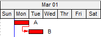
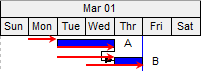
While there is nothing inherently “wrong” with this activity delay model, this example reveals some glaring weaknesses. First, the model assigns delay – two delays, in fact – to activity B, even though B started as soon as its predecessor A would allow, and had an actual duration exactly equal to its forecast duration. B’s dates did not change due to a flaw in its execution, but merely to accommodate the delayed finish of activity A.
Second, the model treats an activity’s start and finish delay as independent phenomena, when there is a clear dependency between them. For example, activity A has a two-day finish delay, of which one day is from an increased duration, and one day is from a late start – but the latter is already reflected in the activity’s start delay!
What would a more useful activity delay model look like? To address the first problem, rather than compare an activity’s start date to its previous start date, we’ll compare its start date to the earliest date its predecessor logic allows it to start, given any delay/recovery to preceding activities.
In the example, activity B’s earliest possible start date is Thursday, due to the delay of its predecessor A. Since Thursday is when B actually started, it has no start delay under our revised model.
To address the second problem, we observe that while there is a dependency between an activity’s start and finish date (which leads to some degree of redundancy when measuring delay), there is no dependency between an activity’s start date and its duration. Thus, instead of recording start delays and finish delays, we will measure start delays and duration delays. To annotate a duration delay (or recovery), we’ll draw an arrow from where the activity would have finished if it kept its original duration to where it actually finishes given its new duration.
Applying both of these improvements, here is what the example scenario would look like under the new delay model:
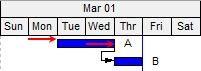
Much better! Activity B, which executed perfectly, is no longer saddled with any form of delay, and activity A’s overall delay has been broken into two independent delays: a one-day start delay, and a one-day duration delay.
Let’s briefly linger on what it means for A’s start delay to be independent from its duration delay. If these delays are truly independent, then it should be possible to “undo” one delay (as part of some counterfactual exercise) without disturbing the other. In this example, what would it look like if A’s duration delay did not happen?
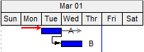
Here, we’ve grayed out A’s duration arrow to show that its duration delay is no longer being applied; that is, A retains its original duration of one day. As a result, B can start (and finish) one day earlier. Despite this alteration of the schedule, A’s one-day start delay remains active, and its interpretation (“activity A started one day later than it should have”) is unchanged.
What if we deactivated A’s start delay instead?
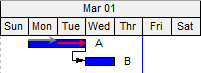
Here, A’s start arrow is grayed out, and its start delay is no longer active. As a result, A starts one day earlier, which allows B to start one day earlier in turn. However, A’s duration arrow remains active, and it continues to signal that A’s duration is one day greater than it was previously. Note that since A starts earlier, the duration delay arrow must now be drawn on Tuesday rather than Wednesday, but this is a superficial difference: duration delay only concerns itself with how far the activity’s finish extends relative to its start, not where that extension occurs in absolute terms. Thus, the removal of A’s start delay has not affected the interpretation of its duration delay.
This level of independence between start and duration delays will prove critical when we introduce the delay impact model in the next section.
Here’s another example of our improved delay model in action:
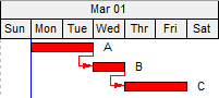
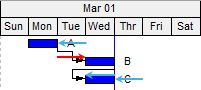
This scenario introduces the notion of start and duration recovery. To begin, activity A was forecast to take two days, but ended up taking only one. As with duration delay, we annotate this by drawing an arrow from where it would have ended with the original duration to where it actually ends with the new duration. Since this is a recovery, the resulting arrow points to the left, and we color it light blue to make it even more visually distinct from a delay arrow.
Since A finished earlier than forecast, its successor, activity B, could have started earlier than forecast – on Tuesday, rather than Wednesday – but it did not. Thus, even though B’s forecast and actual start are the same, we understand that B suffered a one-day start delay, which we represent with a delay arrow pointing from A’s finish on Monday (which is when B could have started) to Wednesday (which is when B actually started).
Next, although activity C is a finish-to-start successor of B, C actually started before B finished. This out-of-sequence execution is the typical way that start recovery occurs in our model; here, we draw an arrow from B’s finish at the end of Wednesday (the earliest that C should have started) to the start of Wednesday (when C actually started, in violation of the FS relationship).
Finally, activity C also saw a one-day duration recovery in addition to its start recovery, rendered in the same manner as A’s duration recovery. This illustrates that start and duration recoveries are independent in the same way that start and duration delays are independent: in particular, the interpretation of a duration arrow does not depend on whether the activity starts in sequence or out-of-sequence.
Delay Impact Model
In a real-world schedule, applying our activity delay model to an analysis window may yield hundreds, if not thousands, of delay and recovery arrows. Many, if not most, of these arrows will be wholly irrelevant in determining why the project as a whole (or some milestone of interest) delayed. Thus, it is vital that we have a way of assessing which arrows are impactful (that is, contribute to the overall project delay), and which are non-impactful (do not contribute). In other words, we need a delay impact model (or just impact model, for short).
A standard axiom in forensic analysis is that a delay is impactful if (and only if) it happens to a critical activity. This may sound like a tautology, given how criticality is typically defined in CPM scheduling. However, traditional descriptions of CPM are based on a single static schedule, but in delay analysis, we are analyzing a dynamic schedule that evolves over time. Thus, a key question that a delay impact model has to answer is, “at what point does an activity need to be critical for its delay to be considered impactful?”
Consider the following analysis window:
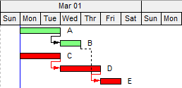
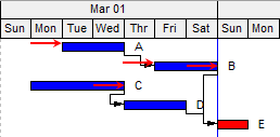
This schedule features two paths, A → B → E and C → D → E, both of which terminate in the same activity E. There is at least one delay arrow on each path. At the start of the window, the longest path in P6 is C → D → E, and at the end of the window, the longest path is simply the activity E.
(In this section, we will treat “critical” and “on a longest path” as synonyms. In general, an activity can be critical without being on a longest path, and a longest path activity can be non-critical, but neither possibility will occur in any of this section’s examples.)
A simple impact model might declare that an arrow is impactful if and only if it happened to an activity that was on a longest path at the start of the window. In this example, since the original longest path is C → D → E, only the duration delay arrow on activity C would be considered impactful; the delay arrows on A and B would be considered non-impactful, as neither activity was on a longest path at period start.
The intuition behind such a model might be that the longest path at the start of the window is the one that the project crew is actually aware of during the window’s execution, and the one that drives on-the-fly decision making. While that idea can be critiqued on purely philosophical grounds, in this example there is also a vexing practical issue: the project finish date suffered a two-day delay, but only one of those days can be accounted for with C’s duration delay.
Indeed, we can’t fully explain the full two-day project variance without looking at the other path, A → B → E; activity E could not have started before Sunday because B just finished at the end of Saturday. Intuitively, A → B → E was clearly “more delayed” then C → D → E over the course of the window, and thus its arrows better explain the overall project delay in its totality.
This observation suggests a revised impact model: an arrow is impactful if and only if it happened to an activity that was on a longest path at the end of the window. Unfortunately, this quickly runs into a technical problem: P6 only calculates criticality and longest paths to the right of the data date – actualized activities are never included in longest paths.
This limitation of P6’s scheduling model explains why the end-of-window longest path in our example is solely activity E, rather than A → B → E. This is problematic and could lead a scheduler to compare the starting longest path, C → D → E, to the final longest path, E, conclude that there was no change to the longest path in this period, and assign all impact to activity C’s delay.
In order to salvage our new impact model, which will assign impact to the delays of A and B rather than C, we’ll need to extend the concept of “longest path” so it works to the left of the data date. Fortunately, this is largely straightforward.
We’ll save the full details for a later section, but the key idea is to broaden the notion of driving relationship. To the right of the data date, a relationship is driving if there is no “gap” between predecessor and successor (more formally, if there is nonpositive free float when measured on the successor’s calendar). To the left of the data date, a relationship is driving even if there is a gap – as long the successor doesn’t have a different predecessor relationship with an even smaller gap.
Consider activity E at the end of our example window, reproduced here for convenience:
According to P6, E does not have a driving predecessor relationship in this schedule, as all of its predecessors are complete (to the left of the data date). Rather, E is being driven by the data date itself (set to the beginning of Sunday, Mar 8).
In our extended longest path model, we look to the left of the data date and see that E has two predecessor relationships. Relationship B → E has no gap, but relationship D → E has a one-day gap. Since B → E has no gap, it is a driving relationship. As for D → E, since E has a different predecessor relationship – namely B → E – with a smaller gap, it is not a driving relationship. (If activities A and B were deleted from this schedule, then D → E would be a driving relationship, despite the one-day gap, since that would be the smallest gap among all of E’s predecessor relationships.)
Since E is on a longest path, and since B → E is a driving relationship, activity B is also on a longest path. Next, we consider relationship A → B: it has a one-day gap (end of Wednesday to beginning of Friday), but since it is B’s only predecessor relationship, it is technically B’s smallest predecessor gap. Thus, A → B is also a driving relationship, and activity A is also on a longest path.
At this point, we’ve established that A → B → E is a longest path in this schedule, and also the only longest path (since D → E is not driving, C → D → E is not a longest path). Applying our impact model, we declare that the start delay of activity A is impactful, as are the start and duration delay of activity B; the duration delay of activity C is non-impactful.
This is the delay impact model that SDA’s Arrows Analysis uses. Before we move on, we should note that there is another important category of impact model: ones that attempt to measure criticality not at the beginning or end of the period, but at the precise moment during the period that the activity’s delay occurred.
The analysis framework that SDA launched with – now called Simulation Analysis – uses such an impact model. This analysis begins by inferring how much progress each activity made during the window, as well as the exact times that progress was made. Using this information, a simulation is performed by stepping day-by-day (or sometimes hour-by-hour or minute-by-minute) from the window start to window finish and “playing back” activity progress at the appropriate times. In doing so, we can measure exactly when activities leave or enter longest paths, and base impact assessments on whether the activity was on a longest path at the exact moment of a delay.
Here are the results of the Simulation Analysis for our current example scenario:
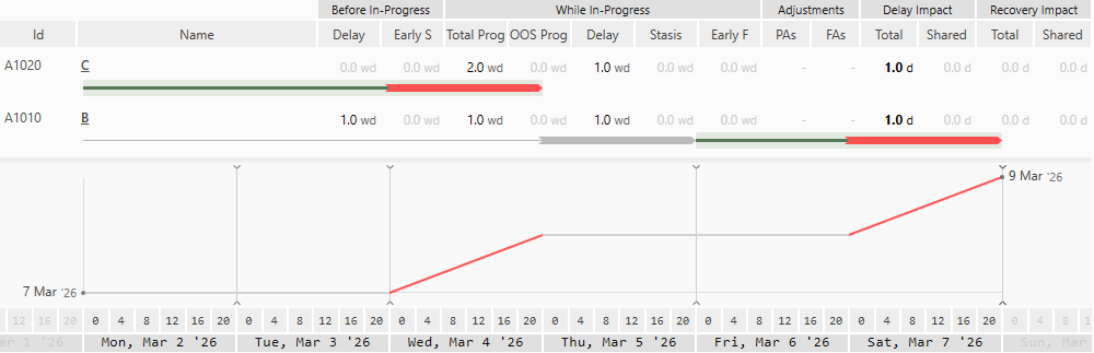
The bottom half of the display is a chart of the Project Finish date over the course of the day-by-day simulation. It shows that the project delayed by one day (from March 7 to March 8) on Wednesday, and by one more day (from March 8 to March 9) on Saturday. Activity C was delaying on Wednesday (duration delay), and C was critical on Wednesday, so C’s delay was assigned the one day of impact measured on Wednesday. Similarly, activity B was critical and delaying on Saturday, so B’s delay was assigned the one day of impact measured on Saturday. Notably, activity A does not appear in the table; A’s start delay happened on the first day of the window (Monday), but A was not yet on the longest path until later in the window, so that delay was assessed as non-impactful.
Unlike the simpler impact models that assigned all impact to either the original longest path C → D → E or the final longest path A → B → E, this model assigns partial impact to each of the paths, using the simulation to determine the moment during the window when the longest path changed.
There are pros and cons to each of the impact models used by Arrows Analysis and Simulation Analysis, and we will contrast the two approaches throughout the remainder of the paper. The largest drawback of the Simulation Analysis is its complexity; given the many rules that drive the simulation, it may not always be completely clear why it took the course that it did. On the other hand, no other analytic approach produces as detailed a set of output; in particular, it not only reports which delays are impactful, but gives a numerical breakdown of how much each individual delay contributed to the overall project delay. In this example, it says that delay to activity C caused 1.0 days of impact, and the delay to activity B caused the other 1.0 days of impact; these impact values sum exactly to the overall 2.0 days of project finish variance.
Arrows Analysis, which uses the simpler impact model, can’t provide a numerical impact breakdown, at least not in the current beta version (Steelray is currently exploring whether it’s possible to augment this style of analysis with numerical breakdowns). It does have some unique strengths, however.
Unlike a typical impact model, Arrows Analysis doesn’t stop after separating impactful activity delays from non-impactful ones. It continues to process the non-impactful delays, looking for delays that would have been impactful, had some other set of delays not happened.
In our current scenario, activity C’s duration delay is a prime example. Because C is not on a longest path at the end of the window, it is technically a non-impactful delay. However, C was on a longest path at the start of the window, which implies that if A and B had not delayed, path C → D → E would have remained a longest path by the end of the window, and C’s delay would have been impactful (and would have caused the project finish to delay by one day, rather than the two days of the original scenario).
This kind of information can be very useful when analyzing concurrency. The party responsible for the delays along path A → B → E may argue that their liability should be offset by the concurrent delays happening along path C → D → E, for example.
Arrows Analysis automatically determines whether a non-impactful activity delay would have been impactful if competing activity paths had not been delayed. This involves yet another model, which we’ll call – for lack of a better name – a “but-for” scheduling model.
A “but-for” scheduling model allows us to compute what a schedule would have looked like if certain activity delays or recoveries had not happened in a given window. As with the other types of models presented so far, there is a degree of subjectivity in how to design one, though the fundamentals are fairly obvious.
We’ll defer the full details of this model to a later section, and instead present the model’s output when asked to remove the three delays on path A → B → E from our example schedule:
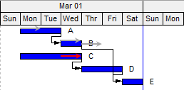
The bottom schedule is the output of the but-for scheduling model. The delay arrows that were “deactivated” by the model are shown in gray. Since A’s start delay was deactivated, A started a day earlier. Since B’s start delay was deactivated, B started immediately after A finished. Since B’s duration delay was deactivated, B’s actual duration was one day instead of two. Finally, since B finished three days earlier than before, activity E could start where D finished, which means that E went from an un-started activity in the real schedule to a complete one in the but-for schedule.
In this modified schedule, the project finish date is now the end of Saturday, one day earlier than before, and the longest path is now C → D → E, which means that C’s duration delay is impactful.
In light of these calculations, Arrows Analysis categorizes activity C’s delay arrow as not as impactful or non-impactful, but rather impactful but-for. Further, it records March 8 as the driven project finish date of the arrow. The driven project finish of an arrow is the project finish date driven by a longest path that the arrow sits on when all parallel delay arrows have been removed.
We’ll see how Arrows Analysis actually presents this information in the next section.
The Arrows Analysis Report
When an Arrows Analysis is performed on a schedule window in SDA, activity delays and recoveries are identified according to the activity delay model, then each delay and recovery is classified as impactful, impactful but-for, or non-impactful according to the delay impact model.
At this point, the activity delays could be presented as a simple list, sorted by impact. However, such a presentation wouldn’t give any insight into why each delay has the impact that it does. To do that, the delays will need to be grouped by path, since impactfulness is largely defined in terms of paths (impactful delays are those on a longest path, and but-for impactful delays are those on a longest path after certain other delays are removed).
Here is what the actual report in SDA looks like for our two-path example scenario:
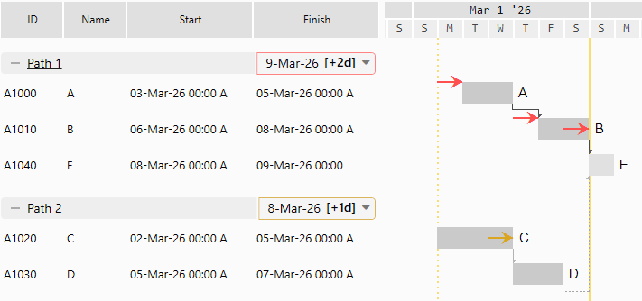
The schedule’s activities have been partitioned into two paths: A → B → E (Path 1) and C → D → E (Path 2). As with the “Multiple Float Paths” feature in P6, when a path is listed, only the activities that are not in any previous path are shown. Thus, even though Path 2 contains activity E, it is not listed under the Path 2 heading, as it was already included under the Path 1 heading. Instead, a relationship arrow is drawn from D up to E, signaling that Path 2 joins back up with Path 1 at activity E. To see the full listing of Path 2, including any parts that are shared with earlier paths, you can click on the “Path 2” hyperlink:
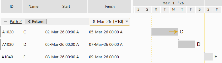
The core activities and core arrows are the activities and arrows that were already present before expanding the path to the full listing. When the path is expanded, the core activities are marked with vertical gray bars at the left edge of the row. In this case, Path 2 contains C, D, and E, but only C and D are core activities.
Recall that under this impact model, each arrow can have a driven project finish date (if that arrow is on a longest path after removing parallel delays from the schedule). When choosing which paths to partition the schedule into, SDA ensures that the following two properties hold for each path:
All of the path’s core arrows have the same driven project finish date.
If the path’s delays are the only delays included (that is, all delays not on the path are removed), the path will be a longest path in the resulting schedule.
Together, these two properties imply that the core activities of a path can be treated as a conceptual unit; that is, each core arrow has the same impactfulness for the same reason (namely, being on the same longest path after certain delays are removed).
In our example, Path 1 is the sole longest path in the schedule. As a longest path, all its arrows are impactful (and thus are colored red), and all have a driven project finish date precisely equal to the end-of-window project finish date (9-Mar-26). Since all of the path’s core arrows share the same driven project finish date, we can treat the driven project finish date as a property of the path itself, and add it to the path’s header. In this case, the exact annotation is “9-Mar-26 [+2d]”, where the “[+2d]” measures the offset from the beginning-of-window project finish date (7-Mar). We circle the annotation in red to emphasize the fact that Path 1 is a longest path.
Thanks to property 1 above, it will always make sense to define and annotate the driven project finish date for any path in the report. Here, the driven project finish date for Path 2 is 8-Mar, since its sole delay arrow’s driven project finish date is 8-Mar. Path 2 is not a longest path, but it is a longest path but-for, so the annotation is circled with yellow, and its impactful but-for delay arrow is also colored yellow.
Clicking on the annotation for Path 2 shows a reminder of how the driven project finish date of 8-Mar-26 was derived; namely, removing all delays not on Path 2, checking to see whether Path 2 is a longest path in the resulting schedule, and if so, what the project finish date is.
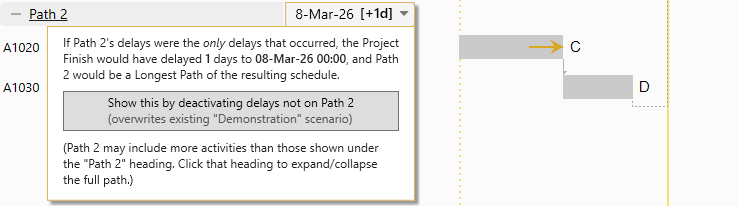
Rather than simply asserting that 8-Mar was the driven project finish date for Path 2, SDA can illustrate this directly, using a “What-If Scenario.” If we click on the tooltip’s button (labelled “Show this by deactivating delays not on Path 2”), SDA will deactivate all delay arrows that are not found on Path 2, then re-calculate the schedule (according to the but-for scheduling model described earlier):
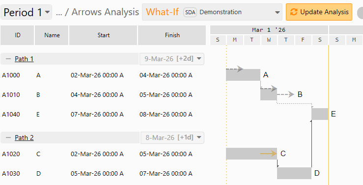
Here we can see that the three arrows of Path 1 are still displayed, but are grayed out and dotted to convey that they are not affecting the schedule in any way. As we saw in earlier sections, removing these delays causes C → D → E to become a longest path, and allows the project finish date to move back by a day (to 8-Mar). In the Gantt diagram, driving relationships are shown as solid lines – black if on a longest path and gray otherwise – and non-driving relationships are shown as dotted lines. We see that removing the Path 1 arrows has caused relationship B → E to become non-driving, and the relationships of Path 2 have become driving (and on the longest path).
The changes made to the schedule (removing the three Path 1 arrows) are encapsulated in a What-If scenario. By clicking the button in the Path’s impact annotation, SDA automatically created a scenario called “Demonstration,” but we can also create and switch between our own scenarios using the What-If dropdown box at the top of the report. No matter what scenario is selected, we can manually remove arrows (or re-enable them) by right clicking them, or by selecting the activity’s table row and toggling the arrow’s “On” checkbox in the drilldown pane:
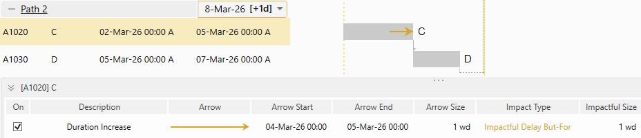
Although the Gantt calculation itself will always remain up-to-date, customizing the schedule with What-If scenarios invalidates the impactfulness of the remaining arrows, as well as the schedule’s path partition (and associated driven project finish dates). In the screenshot above showing the Demonstration scenario, the driven project finish date annotations on the paths are grayed out. If we only wanted to confirm the new project finish date (8-Mar) and the status of C → D → E as the new longest path, we don’t need to go any further. But if we would like to see what the full Arrows Analysis would look like in the absence of the three removed arrows, we can click the “Update Analysis” button at the top of the report:
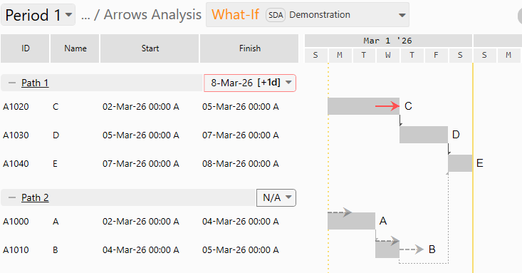
Here, we can see that what was once Path 2 is now Path 1, since C → D → E is now the true longest path in our (modified) schedule, though its driven project finish date is now [+1] instead of [+2]. Further, the duration delay of activity C is now impactful (and shown in red) rather than impactful but-for (yellow).
To cap off this section, let’s consider one more – slightly more realistic – example:
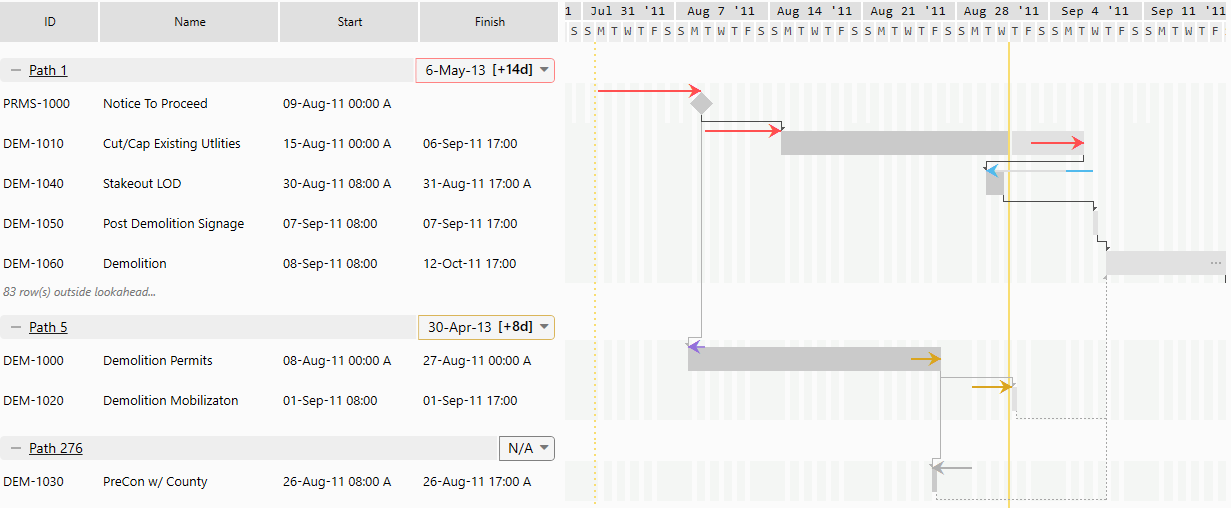
Unlike our previous example, this one includes some recovery arrows. For example, activity DEM-1040 (“Stakeout LOD”) executed out of sequence with its predecessor on Path 1, DEM-1010 (“Cut/Cap Existing Utilities”). Since this arrow is on the longest path, it is impactful, and thus drawn with a light blue color – light blue is to impactful recovery what red is to impactful delay. Note that only part of the recovery arrow is shaded with light blue, with the rest in gray. This signals that all of the out-of-sequence start’s impact was concentrated in the first two days of recovery. This makes sense: in Retained Logic mode, a two-day activity can’t achieve any more recovery impact once it has already started two days early. We will explore this wrinkle of the delay impact model later in the paper.
Meanwhile, DEM-1000 (“Demolition Permits”) also started out of sequence with its predecessor on Path 5, PRMS-1000 (“Notice To Proceed”). Unlike Path 1, Path 5 is not a longest path, so this is not considered an impactful recovery. However, Path 5 is a longest path but-for: if all delays not on Path 5 were removed, Path 5 would be a longest path of the resulting schedule, driving a delay of [+8d] to the project finish. Thus, DEM-1000’s start recovery is deemed impactful but-for, and drawn in purple – purple is to impactful but-for recovery what yellow is to impactful but-for delay.
Finally, consider the recovery arrow on activity DEM-1030 (“PreCon w/ County”). This activity (and arrow) would not be on a longest path if delays on other paths were removed (which can be easily verified with in What-If scenario), and thus the arrow (and Path 276 as a whole) has no driven project finish. The arrow is considered non-impactful and is thus drawn in gray.
Arrows Analysis | Advanced Topics
Coming Soon